Ridge shrinks the directions your data trusts least

Ridge shrinks coefficients most along directions the observed data identifies least reliably.

Published 26 Aug 2026 Updated 04 Sep 2026 9 min read Studied in Advanced Machine Learning, Imperial College London

You only need Ordinary least squares in matrix form, and eigenvalues of a symmetric matrix.

On this page

The usual one-line summary of ridge regression — that it shrinks coefficients toward zero — describes the wrong motion. Fit two standardised predictors correlated at $0.9$ and least squares returns coefficients of $0.895$ and $-0.105$, one strongly positive and one negative, even though both predictors are positively associated with the response. Add a penalty of $\lambda = 10$ and the pair becomes $0.625$ and $0.125$. The gap between them has halved, while their sum has barely moved, from $0.789$ to $0.750$. What the penalty mostly did was pull the two coefficients toward each other, and that asymmetry is the behaviour the one-line summary hides.

What the penalty adds, and to what

Ridge regression minimises the squared error plus a penalty on the squared size of the coefficient vector:

$$ \hat\beta(\lambda) = \arg\min_\beta \; \lVert y - X\beta \rVert_2^2 + \lambda \lVert \beta \rVert_2^2 $$

Here $X$ is the $n \times p$ matrix of standardised predictors, $y$ the response, and $\lambda \ge 0$ the penalty strength you choose. Solving gives a closed form that differs from ordinary least squares by one term 2:

$$ \hat\beta(\lambda) = (X^\top X + \lambda I)^{-1} X^\top y. $$

$X^\top X$ is the cross-product matrix of the predictors, sometimes called the Gram matrix; for standardised columns it is proportional to their sample correlation matrix. Adding $\lambda I$ puts a constant on its diagonal before inversion, which was exactly the point of the original proposal: it makes the inverse exist even when $X^\top X$ is singular or nearly so 1 2.

Adding a constant to a diagonal sounds neutral. It is not, because a fixed constant is enormous next to a small number and negligible next to a large one, and the numbers it lands next to are set by your data rather than by you.

Where the fit is genuinely undetermined

Take the 2×2 system behind the numbers above. Two standardised predictors correlated at $0.9$, measured on 100 observations, give

$$ X^\top X = \begin{pmatrix} 100 & 90 \\ 90 & 100 \end{pmatrix}, \qquad X^\top y = \begin{pmatrix} 80 \\ 70 \end{pmatrix}. $$

An eigenvector of $X^\top X$ is a direction in predictor space that the matrix rescales without rotating, and its eigenvalue is the factor by which it is rescaled. For this matrix the two eigenvectors are the direction in which both coefficients move together and the direction in which they move apart:

$$ q_1 = \tfrac{1}{\sqrt 2}\begin{pmatrix}1\\1\end{pmatrix},\ \ \gamma_1 = 190, \qquad q_2 = \tfrac{1}{\sqrt 2}\begin{pmatrix}1\\-1\end{pmatrix},\ \ \gamma_2 = 10. $$

Read that gap as information. The data constrains “how much of the two predictors together” nineteen times more tightly than it constrains “which of the two.” The consequence is the negative coefficient we started with: a large positive weight on one predictor can be cancelled by a large negative weight on its correlated partner at almost no cost in fit, so least squares picks an arbitrary point along a direction it cannot resolve 2.

One shrinkage factor per direction

Rewriting the estimator in the eigenbasis turns a matrix inverse into a list of independent scalars, one per direction.

Three lines from the closed form to the shrinkage factorderivation

Write the eigendecomposition $X^\top X = Q \Gamma Q^\top$, with $Q$ orthogonal, its columns the eigenvectors $q_j$, and $\Gamma$ diagonal holding the eigenvalues $\gamma_j$. Because $Q Q^\top = I$,

$$ X^\top X + \lambda I = Q(\Gamma + \lambda I)Q^\top \quad\Longrightarrow\quad (X^\top X + \lambda I)^{-1} = Q(\Gamma+\lambda I)^{-1}Q^\top. $$

Writing $c_j = q_j^\top X^\top y$ for the projection of $X^\top y$ onto the $j$-th eigenvector,

$$ \hat\beta(\lambda) = \sum_j \frac{c_j}{\gamma_j + \lambda}\, q_j = \sum_j \frac{\gamma_j}{\gamma_j + \lambda} \cdot \frac{c_j}{\gamma_j}\, q_j. $$

The second form separates the least-squares coefficient $c_j/\gamma_j$ from a multiplier $\gamma_j/(\gamma_j+\lambda)$ that depends only on $\lambda$ and on how large $\gamma_j$ already was.

The Elements of Statistical Learning reaches the same result through the singular value decomposition $X = UDV^\top$ and writes the multiplier as $d_j^2/(d_j^2+\lambda)$, where $d_j$ is the $j$-th singular value of $X$. The two agree because $X^\top X = VD^2V^\top$: the columns of $V$ are the $q_j$ above, and the eigenvalues of $X^\top X$ are the squared singular values, $\gamma_j = d_j^2$ 2.

In words: ridge leaves the least-squares answer alone along each direction and then multiplies it by a number between 0 and 1. That number is close to 1 when the eigenvalue is large relative to $\lambda$ and close to 0 when it is small. Greater shrinkage falls on the directions with the smaller eigenvalues, which are the directions along which the predictors vary least and the fit is therefore least well determined 2.

For the two directions in this example, the multipliers diverge almost immediately:

λ	joint direction, $\frac{190}{190+\lambda}$	contrast direction, $\frac{10}{10+\lambda}$	resulting $(\hat\beta_1, \hat\beta_2)$
0	1.00	1.00	(0.895, −0.105)
10	0.95	0.50	(0.625, 0.125)
50	0.79	0.17	(0.396, 0.229)
190	0.50	0.05	(0.222, 0.172)

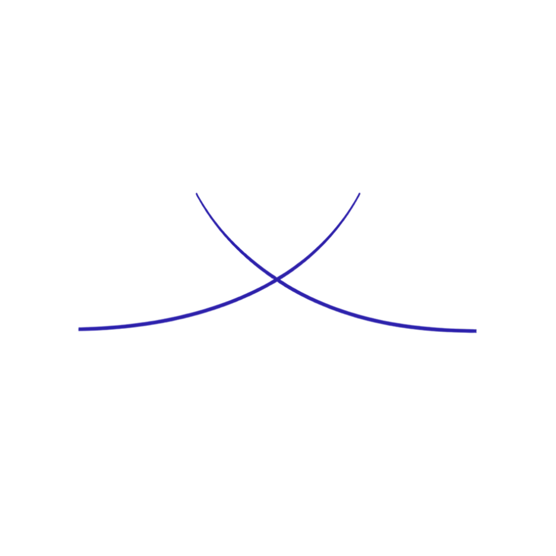
At $\lambda = 10$ the joint direction has lost 5% of its length and the contrast direction has lost half of its own. By $\lambda = 190$ the contrast has been cut to a twentieth while the joint direction retains half. The convergence you can watch in the figure is not ridge preferring similar coefficients. It is the contrast direction being dismantled first, leaving the shared component as most of what survives.

Rescale a column and you have changed the penalty Least squares is scale equivariant: multiply a predictor by $c$ and its coefficient divides by $c$, leaving the fitted values untouched. Ridge estimates do not behave that way, and the fitted contribution of one predictor can shift when a different predictor is rescaled 3. The reason is visible in the table above, since rescaling a column changes the eigenvalues and therefore changes every multiplier. Standardise the predictors before fitting, or the units you happened to record become an undeclared part of the penalty 2 3. For the same family of reasons the intercept is conventionally left unpenalised: shrinking it would make the fit depend on where the origin of $y$ sits 2 3.

Reading a ridge coefficient under collinearity

The practical consequence is a limit on interpretation. Under strong collinearity a single ridge coefficient carries little information on its own, while the group total carries most of what the data actually determined. Ridge returns two similar middling numbers where least squares returned one large and one negative. Neither pair is more correct than the other; least squares chose an arbitrary point along an unresolved direction, and ridge chose a more stable one, buying lower variance at the cost of some bias 3.

If the question is which of two correlated predictors matters, no value of $\lambda$ will answer it. Ridge distributes weight across a correlated group by construction. Answering that question needs either data that breaks the correlation or a method willing to make a discrete choice, such as the lasso.

Two predictors have correlation 0.95. What happens to their coefficients as λ grows?Recall

They converge on each other faster than either approaches zero. Higher correlation makes the contrast direction’s eigenvalue smaller, so the multiplier $\gamma/(\gamma+\lambda)$ collapses for that direction at a penalty small enough to leave the joint direction almost intact.

When is ridge the wrong tool for correlated predictors?Recall

When you need to identify which predictor in a correlated group is responsible. Ridge spreads weight across the group rather than selecting within it. Use the lasso or elastic net if selection is the goal, or collect data that breaks the correlation.

Sources and further reading

Ridge Regression: Biased Estimation for Nonorthogonal Problems (external source) Arthur E. Hoerl & Robert W. Kennard Technometrics 12(1), 55–67 1970
Used for: The original proposal to add a constant to the diagonal of the cross-product matrix before inverting it.
The Elements of Statistical Learning, 2nd edition, §3.4.1 (external source) Trevor Hastie, Robert Tibshirani & Jerome Friedman Springer; full text free from the authors 2009
Used for: The singular-value view of ridge, the shrinkage factor applied to each direction, the cancellation behaviour of correlated predictors, non-equivariance under rescaling, and the unpenalised intercept.
An Introduction to Statistical Learning, 2nd edition, §6.2.1 (external source) Gareth James, Daniela Witten, Trevor Hastie & Robert Tibshirani Springer; full text free from statlearning.com 2021
Used for: The accessible statement that ridge estimates are not scale equivariant, the recommendation to standardise predictors first, and the bias–variance reading of the penalty.