A better fit on your training data can predict worse

Lower training error can mean worse unseen predictions when extra flexibility starts fitting noise.

Published 26 Aug 2026 Updated 04 Sep 2026 9 min read Studied in Machine Learning, Imperial College London

You only need What least-squares regression fits, and what a training/test split is.

On this page

Which of two fitted curves should you trust: the one that misses many of your data points, or the one that passes almost exactly through them all? The second answer is the intuitive one, and here it is wrong. A degree-2 polynomial through nine noisy points of discount percentage against conversion lift leaves a training mean squared error of 2.88; pushing to degree 7 threads the curve through nearly every point and drops that to 1.34. On eight held-out points the ranking reverses: degree 2 scores 2.29 and degree 7 scores 4.13. The fit that looks better on the data it was given is the one to discard.

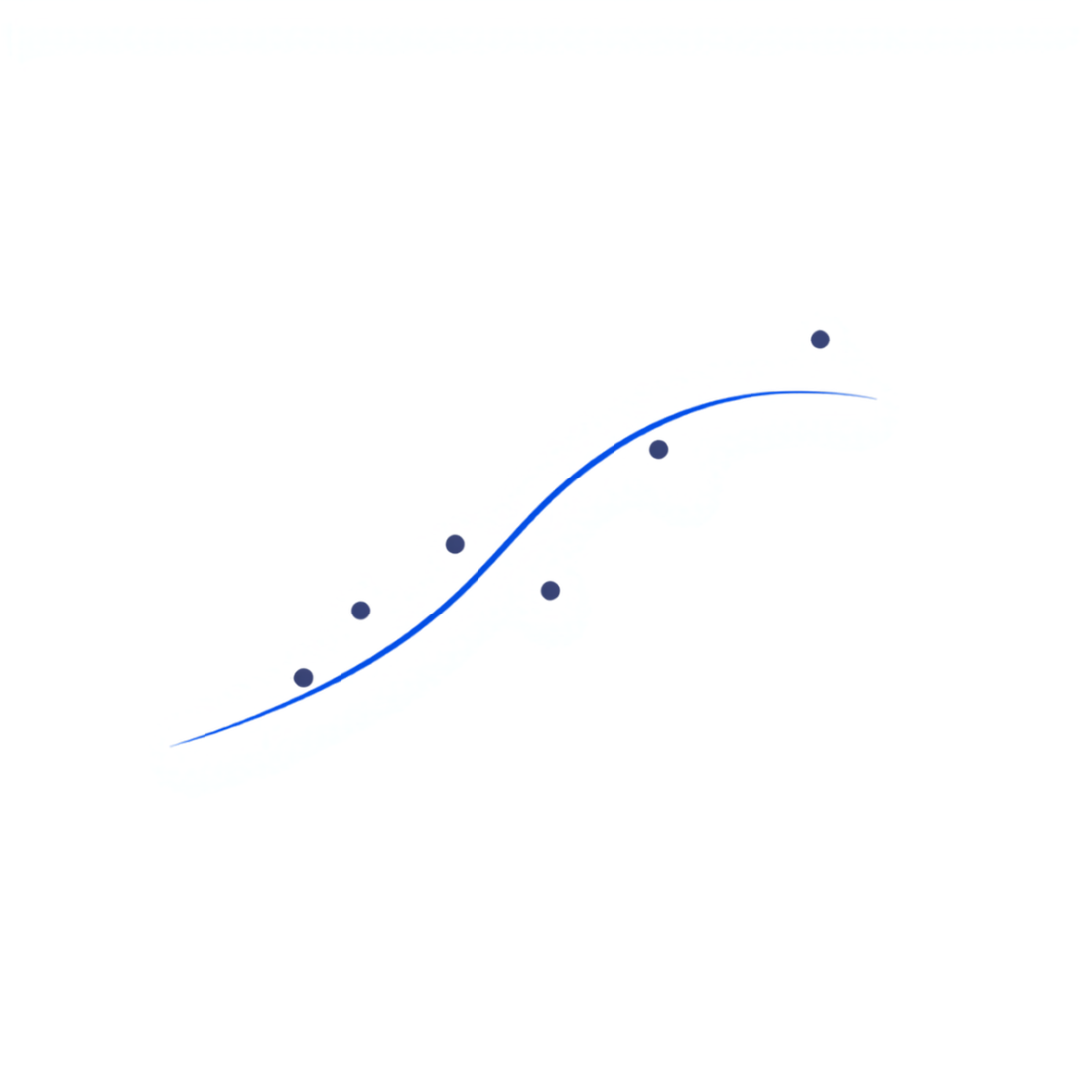
Seven polynomial fits to the same nine points

The data here is synthetic, which is what makes the comparison legible: the relationship the points were generated from is

$$ f(x) = 20 + 1.4x - 0.03x^2 $$

a single-peaked curve where lift rises with the discount and then falls as heavy discounts start reading as a signal of low quality. Nine training points sit at $x = 0, 5, 10, \dots, 40$ with fixed, deliberately chosen noise added. Eight test points sit at the midpoints between them, $x = 2.5, 7.5, \dots, 37.5$, with their own fixed noise. Both sets are held constant so that the only thing changing between rows below is the degree of the fitted polynomial. Errors are mean squared errors in the units of lift, squared.

Degree	Train MSE	Test MSE
1	23.47	15.33
2	2.88	2.29
3	2.83	2.57
4	1.85	2.94
5	1.82	3.18
6	1.34	4.29
7	1.34	4.13

Training error never rises as the degree increases, and that is guaranteed rather than lucky: every degree-$d$ polynomial is also a degree-$(d{+}1)$ polynomial with a zero leading coefficient, so the larger family can match the smaller family’s fit and then look for something better. Test error behaves differently. It reaches its minimum at degree 2, the order of the curve that generated the data, and by degree 7 it is about 80% higher.

The degree-2 fit recovers coefficients of $19.55$, $1.448$ and $-0.0310$ against the true $20$, $1.4$ and $-0.03$. Degree 2 was not chosen to flatter the example. It is the smallest degree with enough freedom to represent the generating curve, and nothing above it has any signal left to find.

Three sources of error, one of which you cannot touch

Suppose the response is $y = f(x) + \varepsilon$ with $\mathbb{E}[\varepsilon] = 0$ and $\mathrm{Var}(\varepsilon) = \sigma^2$, and that $\hat f$ has been fitted to a training set drawn at random. At a single input $x$, the expected squared prediction error splits into three non-negative pieces 2 3:

$$ \mathbb{E}\big[(y - \hat f(x))^2\big] = \underbrace{\big(f(x) - \mathbb{E}[\hat f(x)]\big)^2}_{\text{bias}^2} + \underbrace{\mathrm{Var}\big[\hat f(x)\big]}_{\text{variance}} + \sigma^2 $$

Bias measures how far the model’s average prediction sits from the truth, averaging over training sets. A model too rigid to represent the real relationship stays wrong there no matter how much data arrives. Variance measures how much the prediction at that same point would move if the model were refitted on a different sample from the same process 3. It says nothing about how spread out the data is. The last term, $\sigma^2$, is the variance of the noise in the outcome itself, and no fitting procedure removes it, so the expected test error cannot fall below it 3.

Training error only responds to the first of the three. That is why it kept falling in the table while test error turned around.

Where the three terms come fromderivation

Write $y = f(x) + \varepsilon$ with $\mathbb{E}[\varepsilon] = 0$, $\mathrm{Var}(\varepsilon) = \sigma^2$, and $\varepsilon$ independent of the training set $D$ that $\hat f$ was fitted on. Let $\bar f(x) = \mathbb{E}_D[\hat f(x)]$ be the average prediction over all possible training sets. Then

$$ \mathbb{E}\big[(y-\hat f(x))^2\big] = \mathbb{E}\big[(f(x)+\varepsilon-\hat f(x))^2\big]. $$

Add and subtract $\bar f(x)$ inside the square:

$$ = \mathbb{E}\Big[\big((f(x)-\bar f(x)) + (\bar f(x)-\hat f(x)) + \varepsilon\big)^2\Big]. $$

$f(x)-\bar f(x)$ is a constant once the average over $D$ has been taken. Expanding gives three squared terms and three cross terms. Each cross term is zero: $\varepsilon$ is mean-zero and independent of $D$, so it has zero covariance with anything built from $\hat f$, and $\mathbb{E}_D[\bar f(x)-\hat f(x)] = 0$ by the definition of $\bar f$. What remains is

$$ \big(f(x)-\bar f(x)\big)^2 + \mathbb{E}\big[(\bar f(x)-\hat f(x))^2\big] + \mathbb{E}[\varepsilon^2] = \text{bias}^2 + \text{variance} + \sigma^2. $$

Nothing in that argument required $\hat f$ to be linear or $\varepsilon$ to be Gaussian, which is why the same three terms appear for any fitting procedure under squared-error loss. Geman, Bienenstock and Doursat used exactly this structure to argue that the trade-off constrains flexible estimators in general rather than any one model family 1.

One split is not an expectation

The decomposition describes an average over training sets. The table describes one training set and one test set, and the difference shows up in the numbers. Test error rises from degree 2 to degree 6 and then falls slightly at degree 7, from 4.29 to 4.13. A decomposition that held pointwise for every fitted model would not permit that wobble; an average over many training sets would smooth it away.

The vocabulary for this is worth keeping straight. The Elements of Statistical Learning writes $\mathrm{Err}_{\mathcal{T}}$ for the test error of a model fitted on one specific training set $\mathcal{T}$, and plain $\mathrm{Err}$ for the expected test error, which averages that quantity over the randomness in the training set as well 2. What a single held-out split reports is an estimate of the first quantity. The claim that more flexibility raises variance and lowers bias is a statement about the second, and both textbooks phrase it as a general tendency rather than a guarantee 2 3.

Two things here are exact rather than tendencies: training error is non-increasing in degree for nested families, and expected test error is bounded below by $\sigma^2$. Everything else in the shape of that curve is a strong regularity, not a law, and one split will show you a noisy version of it.

A different knob from the ridge penalty

The ridge regression note turns a different dial. There the model family is fixed and a penalty pulls the coefficients within it toward zero, buying lower variance for a little bias. Here the family itself grows, because degree 7 can represent everything degree 2 can and a great deal more. Shrinkage and model selection are separate mechanisms for the same purchase, and a production pipeline usually uses both.

Evaluating on the training set cannot see variance at all A model scored only on the data it was fitted to has no way to detect variance, because variance is defined by what would happen on data it has not seen. The Elements of Statistical Learning puts the consequence bluntly: training error drops toward zero as complexity rises, and a model with zero training error is typically overfitted and generalises poorly 2. Held-out data or resampling such as cross-validation is what converts “this fits well” into evidence about “this will predict well.”

Why does training error keep falling as complexity increases, even well past the point of overfitting?Recall

Because each more flexible family contains every function the less flexible one could fit. The larger family can reproduce the smaller family’s solution and then search further, so its training error can only match or beat it. Training error measures fit to data already seen, which is precisely what added flexibility improves.

What exactly is "variance" measuring in the decomposition?Recall

How much the fitted model’s prediction at a given point would change if the model were refitted on a different random sample from the same data-generating process. It is not a measure of how spread out the observed data is.

Why can a single held-out split show test error falling when the model got more flexible?Recall

Because one split estimates the test error of one fitted model, not the expectation over training sets that the decomposition describes. The rise in expected test error with excess flexibility is a tendency; on any particular pair of samples, individual degrees can swap places, as degrees 6 and 7 do here.

Sources and further reading

Neural Networks and the Bias/Variance Dilemma (external source) Stuart Geman, Elie Bienenstock & René Doursat Neural Computation 4(1), 1–58 1992
Used for: The paper that named the bias/variance dilemma and framed it as a constraint on flexible estimators rather than a defect of a particular model.
The Elements of Statistical Learning, 2nd edition, §7.2–§7.3 (external source) Trevor Hastie, Robert Tibshirani & Jerome Friedman Springer; full text free from the authors 2009
Used for: The formal decomposition into irreducible error, squared bias and variance, the distinction between test error for one fixed training set and expected test error, and the behaviour of training error as complexity rises.
An Introduction to Statistical Learning, 2nd edition, §2.2.2 (external source) Gareth James, Daniela Witten, Trevor Hastie & Robert Tibshirani Springer; full text free from statlearning.com 2021
Used for: The definition of expected test MSE as an average over repeated training sets, the plain-language definitions of bias and variance, and the statement that flexibility raises variance and lowers bias only as a general rule.